Technique of integral evaluation
Trigonometry Functions (sin, cos, tan, inverse) Generalized trigonometry Reference Laws and theorems Sines Cosines Tangents Cotangents Calculus Mathematicians
Part of a series of articles about Calculus ∫ a b f ′ ( t ) d t = f ( b ) − f ( a ) {\displaystyle \int _{a}^{b}f'(t)\,dt=f(b)-f(a)} Definitions Integration by
In mathematics , a trigonometric substitution replaces a trigonometric function for another expression. In calculus , trigonometric substitutions are a technique for evaluating integrals. In this case, an expression involving a radical function is replaced with a trigonometric one. Trigonometric identities may help simplify the answer.[1] [2]
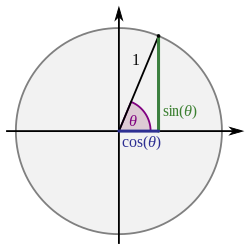
Case I: Integrands containing a 2 − x 2 Let x = a sin θ , {\displaystyle x=a\sin \theta ,} identity 1 − sin 2 θ = cos 2 θ . {\displaystyle 1-\sin ^{2}\theta =\cos ^{2}\theta .}
Examples of Case I Geometric construction for Case I Example 1 In the integral
∫ d x a 2 − x 2 , {\displaystyle \int {\frac {dx}{\sqrt {a^{2}-x^{2}}}},} we may use
x = a sin θ , d x = a cos θ d θ , θ = arcsin x a . {\displaystyle x=a\sin \theta ,\quad dx=a\cos \theta \,d\theta ,\quad \theta =\arcsin {\frac {x}{a}}.} Then,
∫ d x a 2 − x 2 = ∫ a cos θ d θ a 2 − a 2 sin 2 θ = ∫ a cos θ d θ a 2 ( 1 − sin 2 θ ) = ∫ a cos θ d θ a 2 cos 2 θ = ∫ d θ = θ + C = arcsin x a + C . {\displaystyle {\begin{aligned}\int {\frac {dx}{\sqrt {a^{2}-x^{2}}}}&=\int {\frac {a\cos \theta \,d\theta }{\sqrt {a^{2}-a^{2}\sin ^{2}\theta }}}\\[6pt]&=\int {\frac {a\cos \theta \,d\theta }{\sqrt {a^{2}(1-\sin ^{2}\theta )}}}\\[6pt]&=\int {\frac {a\cos \theta \,d\theta }{\sqrt {a^{2}\cos ^{2}\theta }}}\\[6pt]&=\int d\theta \\[6pt]&=\theta +C\\[6pt]&=\arcsin {\frac {x}{a}}+C.\end{aligned}}} The above step requires that a > 0 {\displaystyle a>0} cos θ > 0. {\displaystyle \cos \theta >0.} a {\displaystyle a} a 2 , {\displaystyle a^{2},} − π / 2 < θ < π / 2 {\displaystyle -\pi /2<\theta <\pi /2}
For a definite integral, one must figure out how the bounds of integration change. For example, as x {\displaystyle x} 0 {\displaystyle 0} a / 2 , {\displaystyle a/2,} sin θ {\displaystyle \sin \theta } 0 {\displaystyle 0} 1 / 2 , {\displaystyle 1/2,} θ {\displaystyle \theta } 0 {\displaystyle 0} π / 6. {\displaystyle \pi /6.}
∫ 0 a / 2 d x a 2 − x 2 = ∫ 0 π / 6 d θ = π 6 . {\displaystyle \int _{0}^{a/2}{\frac {dx}{\sqrt {a^{2}-x^{2}}}}=\int _{0}^{\pi /6}d\theta ={\frac {\pi }{6}}.} Some care is needed when picking the bounds. Because integration above requires that − π / 2 < θ < π / 2 {\displaystyle -\pi /2<\theta <\pi /2} θ {\displaystyle \theta } 0 {\displaystyle 0} π / 6. {\displaystyle \pi /6.} θ {\displaystyle \theta } π {\displaystyle \pi } 5 π / 6 , {\displaystyle 5\pi /6,}
Alternatively, fully evaluate the indefinite integrals before applying the boundary conditions. In that case, the antiderivative gives
∫ 0 a / 2 d x a 2 − x 2 = arcsin ( x a ) | 0 a / 2 = arcsin ( 1 2 ) − arcsin ( 0 ) = π 6 {\displaystyle \int _{0}^{a/2}{\frac {dx}{\sqrt {a^{2}-x^{2}}}}=\arcsin \left({\frac {x}{a}}\right){\Biggl |}_{0}^{a/2}=\arcsin \left({\frac {1}{2}}\right)-\arcsin(0)={\frac {\pi }{6}}} as before.
Example 2 The integral
∫ a 2 − x 2 d x , {\displaystyle \int {\sqrt {a^{2}-x^{2}}}\,dx,} may be evaluated by letting x = a sin θ , d x = a cos θ d θ , θ = arcsin x a , {\textstyle x=a\sin \theta ,\,dx=a\cos \theta \,d\theta ,\,\theta =\arcsin {\frac {x}{a}},} a > 0 {\displaystyle a>0} a 2 = a , {\textstyle {\sqrt {a^{2}}}=a,} − π 2 ≤ θ ≤ π 2 {\textstyle -{\frac {\pi }{2}}\leq \theta \leq {\frac {\pi }{2}}} cos θ ≥ 0 {\displaystyle \cos \theta \geq 0} cos 2 θ = cos θ . {\textstyle {\sqrt {\cos ^{2}\theta }}=\cos \theta .}
Then,
∫ a 2 − x 2 d x = ∫ a 2 − a 2 sin 2 θ ( a cos θ ) d θ = ∫ a 2 ( 1 − sin 2 θ ) ( a cos θ ) d θ = ∫ a 2 ( cos 2 θ ) ( a cos θ ) d θ = ∫ ( a cos θ ) ( a cos θ ) d θ = a 2 ∫ cos 2 θ d θ = a 2 ∫ ( 1 + cos 2 θ 2 ) d θ = a 2 2 ( θ + 1 2 sin 2 θ ) + C = a 2 2 ( θ + sin θ cos θ ) + C = a 2 2 ( arcsin x a + x a 1 − x 2 a 2 ) + C = a 2 2 arcsin x a + x 2 a 2 − x 2 + C . {\displaystyle {\begin{aligned}\int {\sqrt {a^{2}-x^{2}}}\,dx&=\int {\sqrt {a^{2}-a^{2}\sin ^{2}\theta }}\,(a\cos \theta )\,d\theta \\[6pt]&=\int {\sqrt {a^{2}(1-\sin ^{2}\theta )}}\,(a\cos \theta )\,d\theta \\[6pt]&=\int {\sqrt {a^{2}(\cos ^{2}\theta )}}\,(a\cos \theta )\,d\theta \\[6pt]&=\int (a\cos \theta )(a\cos \theta )\,d\theta \\[6pt]&=a^{2}\int \cos ^{2}\theta \,d\theta \\[6pt]&=a^{2}\int \left({\frac {1+\cos 2\theta }{2}}\right)\,d\theta \\[6pt]&={\frac {a^{2}}{2}}\left(\theta +{\frac {1}{2}}\sin 2\theta \right)+C\\[6pt]&={\frac {a^{2}}{2}}(\theta +\sin \theta \cos \theta )+C\\[6pt]&={\frac {a^{2}}{2}}\left(\arcsin {\frac {x}{a}}+{\frac {x}{a}}{\sqrt {1-{\frac {x^{2}}{a^{2}}}}}\right)+C\\[6pt]&={\frac {a^{2}}{2}}\arcsin {\frac {x}{a}}+{\frac {x}{2}}{\sqrt {a^{2}-x^{2}}}+C.\end{aligned}}} For a definite integral, the bounds change once the substitution is performed and are determined using the equation θ = arcsin x a , {\textstyle \theta =\arcsin {\frac {x}{a}},} − π 2 ≤ θ ≤ π 2 . {\textstyle -{\frac {\pi }{2}}\leq \theta \leq {\frac {\pi }{2}}.}
For example, the definite integral
∫ − 1 1 4 − x 2 d x , {\displaystyle \int _{-1}^{1}{\sqrt {4-x^{2}}}\,dx,} may be evaluated by substituting x = 2 sin θ , d x = 2 cos θ d θ , {\displaystyle x=2\sin \theta ,\,dx=2\cos \theta \,d\theta ,} θ = arcsin x 2 . {\textstyle \theta =\arcsin {\frac {x}{2}}.}
Because arcsin ( 1 / 2 ) = π / 6 {\displaystyle \arcsin(1/{2})=\pi /6} arcsin ( − 1 / 2 ) = − π / 6 , {\displaystyle \arcsin(-1/2)=-\pi /6,}
∫ − 1 1 4 − x 2 d x = ∫ − π / 6 π / 6 4 − 4 sin 2 θ ( 2 cos θ ) d θ = ∫ − π / 6 π / 6 4 ( 1 − sin 2 θ ) ( 2 cos θ ) d θ = ∫ − π / 6 π / 6 4 ( cos 2 θ ) ( 2 cos θ ) d θ = ∫ − π / 6 π / 6 ( 2 cos θ ) ( 2 cos θ ) d θ = 4 ∫ − π / 6 π / 6 cos 2 θ d θ = 4 ∫ − π / 6 π / 6 ( 1 + cos 2 θ 2 ) d θ = 2 [ θ + 1 2 sin 2 θ ] − π / 6 π / 6 = [ 2 θ + sin 2 θ ] | − π / 6 π / 6 = ( π 3 + sin π 3 ) − ( − π 3 + sin ( − π 3 ) ) = 2 π 3 + 3 . {\displaystyle {\begin{aligned}\int _{-1}^{1}{\sqrt {4-x^{2}}}\,dx&=\int _{-\pi /6}^{\pi /6}{\sqrt {4-4\sin ^{2}\theta }}\,(2\cos \theta )\,d\theta \\[6pt]&=\int _{-\pi /6}^{\pi /6}{\sqrt {4(1-\sin ^{2}\theta )}}\,(2\cos \theta )\,d\theta \\[6pt]&=\int _{-\pi /6}^{\pi /6}{\sqrt {4(\cos ^{2}\theta )}}\,(2\cos \theta )\,d\theta \\[6pt]&=\int _{-\pi /6}^{\pi /6}(2\cos \theta )(2\cos \theta )\,d\theta \\[6pt]&=4\int _{-\pi /6}^{\pi /6}\cos ^{2}\theta \,d\theta \\[6pt]&=4\int _{-\pi /6}^{\pi /6}\left({\frac {1+\cos 2\theta }{2}}\right)\,d\theta \\[6pt]&=2\left[\theta +{\frac {1}{2}}\sin 2\theta \right]_{-\pi /6}^{\pi /6}=[2\theta +\sin 2\theta ]{\Biggl |}_{-\pi /6}^{\pi /6}\\[6pt]&=\left({\frac {\pi }{3}}+\sin {\frac {\pi }{3}}\right)-\left(-{\frac {\pi }{3}}+\sin \left(-{\frac {\pi }{3}}\right)\right)={\frac {2\pi }{3}}+{\sqrt {3}}.\end{aligned}}} On the other hand, direct application of the boundary terms to the previously obtained formula for the antiderivative yields
∫ − 1 1 4 − x 2 d x = [ 2 2 2 arcsin x 2 + x 2 2 2 − x 2 ] − 1 1 = ( 2 arcsin 1 2 + 1 2 4 − 1 ) − ( 2 arcsin ( − 1 2 ) + − 1 2 4 − 1 ) = ( 2 ⋅ π 6 + 3 2 ) − ( 2 ⋅ ( − π 6 ) − 3 2 ) = 2 π 3 + 3 {\displaystyle {\begin{aligned}\int _{-1}^{1}{\sqrt {4-x^{2}}}\,dx&=\left[{\frac {2^{2}}{2}}\arcsin {\frac {x}{2}}+{\frac {x}{2}}{\sqrt {2^{2}-x^{2}}}\right]_{-1}^{1}\\[6pt]&=\left(2\arcsin {\frac {1}{2}}+{\frac {1}{2}}{\sqrt {4-1}}\right)-\left(2\arcsin \left(-{\frac {1}{2}}\right)+{\frac {-1}{2}}{\sqrt {4-1}}\right)\\[6pt]&=\left(2\cdot {\frac {\pi }{6}}+{\frac {\sqrt {3}}{2}}\right)-\left(2\cdot \left(-{\frac {\pi }{6}}\right)-{\frac {\sqrt {3}}{2}}\right)\\[6pt]&={\frac {2\pi }{3}}+{\sqrt {3}}\end{aligned}}} as before.
Case II: Integrands containing a 2 + x 2 Let x = a tan θ , {\displaystyle x=a\tan \theta ,} 1 + tan 2 θ = sec 2 θ . {\displaystyle 1+\tan ^{2}\theta =\sec ^{2}\theta .}
Examples of Case II Geometric construction for Case II Example 1 In the integral
∫ d x a 2 + x 2 {\displaystyle \int {\frac {dx}{a^{2}+x^{2}}}} we may write
x = a tan θ , d x = a sec 2 θ d θ , θ = arctan x a , {\displaystyle x=a\tan \theta ,\quad dx=a\sec ^{2}\theta \,d\theta ,\quad \theta =\arctan {\frac {x}{a}},} so that the integral becomes
∫ d x a 2 + x 2 = ∫ a sec 2 θ d θ a 2 + a 2 tan 2 θ = ∫ a sec 2 θ d θ a 2 ( 1 + tan 2 θ ) = ∫ a sec 2 θ d θ a 2 sec 2 θ = ∫ d θ a = θ a + C = 1 a arctan x a + C , {\displaystyle {\begin{aligned}\int {\frac {dx}{a^{2}+x^{2}}}&=\int {\frac {a\sec ^{2}\theta \,d\theta }{a^{2}+a^{2}\tan ^{2}\theta }}\\[6pt]&=\int {\frac {a\sec ^{2}\theta \,d\theta }{a^{2}(1+\tan ^{2}\theta )}}\\[6pt]&=\int {\frac {a\sec ^{2}\theta \,d\theta }{a^{2}\sec ^{2}\theta }}\\[6pt]&=\int {\frac {d\theta }{a}}\\[6pt]&={\frac {\theta }{a}}+C\\[6pt]&={\frac {1}{a}}\arctan {\frac {x}{a}}+C,\end{aligned}}} provided a ≠ 0. {\displaystyle a\neq 0.}
For a definite integral, the bounds change once the substitution is performed and are determined using the equation θ = arctan x a , {\displaystyle \theta =\arctan {\frac {x}{a}},} − π 2 < θ < π 2 . {\displaystyle -{\frac {\pi }{2}}<\theta <{\frac {\pi }{2}}.}
For example, the definite integral
∫ 0 1 4 d x 1 + x 2 {\displaystyle \int _{0}^{1}{\frac {4\,dx}{1+x^{2}}}\,} may be evaluated by substituting x = tan θ , d x = sec 2 θ d θ , {\displaystyle x=\tan \theta ,\,dx=\sec ^{2}\theta \,d\theta ,} θ = arctan x . {\displaystyle \theta =\arctan x.}
Since arctan 0 = 0 {\displaystyle \arctan 0=0} arctan 1 = π / 4 , {\displaystyle \arctan 1=\pi /4,}
∫ 0 1 4 d x 1 + x 2 = 4 ∫ 0 1 d x 1 + x 2 = 4 ∫ 0 π / 4 sec 2 θ d θ 1 + tan 2 θ = 4 ∫ 0 π / 4 sec 2 θ d θ sec 2 θ = 4 ∫ 0 π / 4 d θ = ( 4 θ ) | 0 π / 4 = 4 ( π 4 − 0 ) = π . {\displaystyle {\begin{aligned}\int _{0}^{1}{\frac {4\,dx}{1+x^{2}}}&=4\int _{0}^{1}{\frac {dx}{1+x^{2}}}\\[6pt]&=4\int _{0}^{\pi /4}{\frac {\sec ^{2}\theta \,d\theta }{1+\tan ^{2}\theta }}\\[6pt]&=4\int _{0}^{\pi /4}{\frac {\sec ^{2}\theta \,d\theta }{\sec ^{2}\theta }}\\[6pt]&=4\int _{0}^{\pi /4}d\theta \\[6pt]&=(4\theta ){\Bigg |}_{0}^{\pi /4}=4\left({\frac {\pi }{4}}-0\right)=\pi .\end{aligned}}} Meanwhile, direct application of the boundary terms to the formula for the antiderivative yields
∫ 0 1 4 d x 1 + x 2 = 4 ∫ 0 1 d x 1 + x 2 = 4 [ 1 1 arctan x 1 ] 0 1 = 4 ( arctan x ) | 0 1 = 4 ( arctan 1 − arctan 0 ) = 4 ( π 4 − 0 ) = π , {\displaystyle {\begin{aligned}\int _{0}^{1}{\frac {4\,dx}{1+x^{2}}}\,&=4\int _{0}^{1}{\frac {dx}{1+x^{2}}}\\&=4\left[{\frac {1}{1}}\arctan {\frac {x}{1}}\right]_{0}^{1}\\&=4(\arctan x){\Bigg |}_{0}^{1}\\&=4(\arctan 1-\arctan 0)\\&=4\left({\frac {\pi }{4}}-0\right)=\pi ,\end{aligned}}} same as before.
Example 2 The integral
∫ a 2 + x 2 d x {\displaystyle \int {\sqrt {a^{2}+x^{2}}}\,{dx}} may be evaluated by letting x = a tan θ , d x = a sec 2 θ d θ , θ = arctan x a , {\displaystyle x=a\tan \theta ,\,dx=a\sec ^{2}\theta \,d\theta ,\,\theta =\arctan {\frac {x}{a}},}
where a > 0 {\displaystyle a>0} a 2 = a , {\displaystyle {\sqrt {a^{2}}}=a,} − π 2 < θ < π 2 {\displaystyle -{\frac {\pi }{2}}<\theta <{\frac {\pi }{2}}} sec θ > 0 {\displaystyle \sec \theta >0} sec 2 θ = sec θ . {\displaystyle {\sqrt {\sec ^{2}\theta }}=\sec \theta .}
Then,
∫ a 2 + x 2 d x = ∫ a 2 + a 2 tan 2 θ ( a sec 2 θ ) d θ = ∫ a 2 ( 1 + tan 2 θ ) ( a sec 2 θ ) d θ = ∫ a 2 sec 2 θ ( a sec 2 θ ) d θ = ∫ ( a sec θ ) ( a sec 2 θ ) d θ = a 2 ∫ sec 3 θ d θ . {\displaystyle {\begin{aligned}\int {\sqrt {a^{2}+x^{2}}}\,dx&=\int {\sqrt {a^{2}+a^{2}\tan ^{2}\theta }}\,(a\sec ^{2}\theta )\,d\theta \\[6pt]&=\int {\sqrt {a^{2}(1+\tan ^{2}\theta )}}\,(a\sec ^{2}\theta )\,d\theta \\[6pt]&=\int {\sqrt {a^{2}\sec ^{2}\theta }}\,(a\sec ^{2}\theta )\,d\theta \\[6pt]&=\int (a\sec \theta )(a\sec ^{2}\theta )\,d\theta \\[6pt]&=a^{2}\int \sec ^{3}\theta \,d\theta .\\[6pt]\end{aligned}}} The
integral of secant cubed may be evaluated using
integration by parts . As a result,
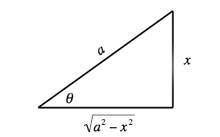
∫ a 2 + x 2 d x = a 2 2 ( sec θ tan θ + ln | sec θ + tan θ | ) + C = a 2 2 ( 1 + x 2 a 2 ⋅ x a + ln | 1 + x 2 a 2 + x a | ) + C = 1 2 ( x a 2 + x 2 + a 2 ln | x + a 2 + x 2 a | ) + C . {\displaystyle {\begin{aligned}\int {\sqrt {a^{2}+x^{2}}}\,dx&={\frac {a^{2}}{2}}(\sec \theta \tan \theta +\ln |\sec \theta +\tan \theta |)+C\\[6pt]&={\frac {a^{2}}{2}}\left({\sqrt {1+{\frac {x^{2}}{a^{2}}}}}\cdot {\frac {x}{a}}+\ln \left|{\sqrt {1+{\frac {x^{2}}{a^{2}}}}}+{\frac {x}{a}}\right|\right)+C\\[6pt]&={\frac {1}{2}}\left(x{\sqrt {a^{2}+x^{2}}}+a^{2}\ln \left|{\frac {x+{\sqrt {a^{2}+x^{2}}}}{a}}\right|\right)+C.\end{aligned}}} Case III: Integrands containing x 2 − a 2 Let x = a sec θ , {\displaystyle x=a\sec \theta ,} sec 2 θ − 1 = tan 2 θ . {\displaystyle \sec ^{2}\theta -1=\tan ^{2}\theta .}
Examples of Case III Geometric construction for Case III Integrals such as
∫ d x x 2 − a 2 {\displaystyle \int {\frac {dx}{x^{2}-a^{2}}}} can also be evaluated by partial fractions rather than trigonometric substitutions. However, the integral
∫ x 2 − a 2 d x {\displaystyle \int {\sqrt {x^{2}-a^{2}}}\,dx} cannot. In this case, an appropriate substitution is:
x = a sec θ , d x = a sec θ tan θ d θ , θ = arcsec x a , {\displaystyle x=a\sec \theta ,\,dx=a\sec \theta \tan \theta \,d\theta ,\,\theta =\operatorname {arcsec} {\frac {x}{a}},} where a > 0 {\displaystyle a>0} a 2 = a , {\displaystyle {\sqrt {a^{2}}}=a,} 0 ≤ θ < π 2 {\displaystyle 0\leq \theta <{\frac {\pi }{2}}} x > 0 , {\displaystyle x>0,} tan θ ≥ 0 {\displaystyle \tan \theta \geq 0} tan 2 θ = tan θ . {\displaystyle {\sqrt {\tan ^{2}\theta }}=\tan \theta .}
Then,
∫ x 2 − a 2 d x = ∫ a 2 sec 2 θ − a 2 ⋅ a sec θ tan θ d θ = ∫ a 2 ( sec 2 θ − 1 ) ⋅ a sec θ tan θ d θ = ∫ a 2 tan 2 θ ⋅ a sec θ tan θ d θ = ∫ a 2 sec θ tan 2 θ d θ = a 2 ∫ ( sec θ ) ( sec 2 θ − 1 ) d θ = a 2 ∫ ( sec 3 θ − sec θ ) d θ . {\displaystyle {\begin{aligned}\int {\sqrt {x^{2}-a^{2}}}\,dx&=\int {\sqrt {a^{2}\sec ^{2}\theta -a^{2}}}\cdot a\sec \theta \tan \theta \,d\theta \\&=\int {\sqrt {a^{2}(\sec ^{2}\theta -1)}}\cdot a\sec \theta \tan \theta \,d\theta \\&=\int {\sqrt {a^{2}\tan ^{2}\theta }}\cdot a\sec \theta \tan \theta \,d\theta \\&=\int a^{2}\sec \theta \tan ^{2}\theta \,d\theta \\&=a^{2}\int (\sec \theta )(\sec ^{2}\theta -1)\,d\theta \\&=a^{2}\int (\sec ^{3}\theta -\sec \theta )\,d\theta .\end{aligned}}} One may evaluate the integral of the secant function by multiplying the numerator and denominator by ( sec θ + tan θ ) {\displaystyle (\sec \theta +\tan \theta )} integral of secant cubed by parts.[3]
∫ x 2 − a 2 d x = a 2 2 ( sec θ tan θ + ln | sec θ + tan θ | ) − a 2 ln | sec θ + tan θ | + C = a 2 2 ( sec θ tan θ − ln | sec θ + tan θ | ) + C = a 2 2 ( x a ⋅ x 2 a 2 − 1 − ln | x a + x 2 a 2 − 1 | ) + C = 1 2 ( x x 2 − a 2 − a 2 ln | x + x 2 − a 2 a | ) + C . {\displaystyle {\begin{aligned}\int {\sqrt {x^{2}-a^{2}}}\,dx&={\frac {a^{2}}{2}}(\sec \theta \tan \theta +\ln |\sec \theta +\tan \theta |)-a^{2}\ln |\sec \theta +\tan \theta |+C\\[6pt]&={\frac {a^{2}}{2}}(\sec \theta \tan \theta -\ln |\sec \theta +\tan \theta |)+C\\[6pt]&={\frac {a^{2}}{2}}\left({\frac {x}{a}}\cdot {\sqrt {{\frac {x^{2}}{a^{2}}}-1}}-\ln \left|{\frac {x}{a}}+{\sqrt {{\frac {x^{2}}{a^{2}}}-1}}\right|\right)+C\\[6pt]&={\frac {1}{2}}\left(x{\sqrt {x^{2}-a^{2}}}-a^{2}\ln \left|{\frac {x+{\sqrt {x^{2}-a^{2}}}}{a}}\right|\right)+C.\end{aligned}}} When π 2 < θ ≤ π , {\displaystyle {\frac {\pi }{2}}<\theta \leq \pi ,} x < 0 {\displaystyle x<0} tan θ ≤ 0 , {\displaystyle \tan \theta \leq 0,} tan 2 θ = − tan θ {\displaystyle {\sqrt {\tan ^{2}\theta }}=-\tan \theta }
Substitutions that eliminate trigonometric functions Substitution can be used to remove trigonometric functions.
For instance,
∫ f ( sin ( x ) , cos ( x ) ) d x = ∫ 1 ± 1 − u 2 f ( u , ± 1 − u 2 ) d u u = sin ( x ) ∫ f ( sin ( x ) , cos ( x ) ) d x = ∫ 1 ∓ 1 − u 2 f ( ± 1 − u 2 , u ) d u u = cos ( x ) ∫ f ( sin ( x ) , cos ( x ) ) d x = ∫ 2 1 + u 2 f ( 2 u 1 + u 2 , 1 − u 2 1 + u 2 ) d u u = tan ( x 2 ) {\displaystyle {\begin{aligned}\int f(\sin(x),\cos(x))\,dx&=\int {\frac {1}{\pm {\sqrt {1-u^{2}}}}}f\left(u,\pm {\sqrt {1-u^{2}}}\right)\,du&&u=\sin(x)\\[6pt]\int f(\sin(x),\cos(x))\,dx&=\int {\frac {1}{\mp {\sqrt {1-u^{2}}}}}f\left(\pm {\sqrt {1-u^{2}}},u\right)\,du&&u=\cos(x)\\[6pt]\int f(\sin(x),\cos(x))\,dx&=\int {\frac {2}{1+u^{2}}}f\left({\frac {2u}{1+u^{2}}},{\frac {1-u^{2}}{1+u^{2}}}\right)\,du&&u=\tan \left({\tfrac {x}{2}}\right)\\[6pt]\end{aligned}}} The last substitution is known as the Weierstrass substitution , which makes use of tangent half-angle formulas .
For example,
∫ 4 cos x ( 1 + cos x ) 3 d x = ∫ 2 1 + u 2 4 ( 1 − u 2 1 + u 2 ) ( 1 + 1 − u 2 1 + u 2 ) 3 d u = ∫ ( 1 − u 2 ) ( 1 + u 2 ) d u = ∫ ( 1 − u 4 ) d u = u − u 5 5 + C = tan x 2 − 1 5 tan 5 x 2 + C . {\displaystyle {\begin{aligned}\int {\frac {4\cos x}{(1+\cos x)^{3}}}\,dx&=\int {\frac {2}{1+u^{2}}}{\frac {4\left({\frac {1-u^{2}}{1+u^{2}}}\right)}{\left(1+{\frac {1-u^{2}}{1+u^{2}}}\right)^{3}}}\,du=\int (1-u^{2})(1+u^{2})\,du\\&=\int (1-u^{4})\,du=u-{\frac {u^{5}}{5}}+C=\tan {\frac {x}{2}}-{\frac {1}{5}}\tan ^{5}{\frac {x}{2}}+C.\end{aligned}}} Hyperbolic substitution Substitutions of hyperbolic functions can also be used to simplify integrals.[4]
In the integral ∫ d x a 2 + x 2 , {\displaystyle \int {\frac {dx}{\sqrt {a^{2}+x^{2}}}}\,,} x = a sinh u , {\displaystyle x=a\sinh {u},} d x = a cosh u d u . {\displaystyle dx=a\cosh u\,du.}
Then, using the identities cosh 2 ( x ) − sinh 2 ( x ) = 1 {\displaystyle \cosh ^{2}(x)-\sinh ^{2}(x)=1} sinh − 1 x = ln ( x + x 2 + 1 ) , {\displaystyle \sinh ^{-1}{x}=\ln(x+{\sqrt {x^{2}+1}}),}
∫ d x a 2 + x 2 = ∫ a cosh u d u a 2 + a 2 sinh 2 u , = ∫ a cosh u d u a 1 + sinh 2 u = ∫ a cosh u a cosh u d u = u + C = sinh − 1 x a + C = ln ( x 2 a 2 + 1 + x a ) + C = ln ( x 2 + a 2 + x a ) + C {\displaystyle {\begin{aligned}\int {\frac {dx}{\sqrt {a^{2}+x^{2}}}}\,&=\int {\frac {a\cosh u\,du}{\sqrt {a^{2}+a^{2}\sinh ^{2}u}}}\ ,\\[6pt]&=\int {\frac {a\cosh {u}\,du}{a{\sqrt {1+\sinh ^{2}{u}}}}}\,\\[6pt]&=\int {\frac {a\cosh {u}}{a\cosh u}}\,du\\[6pt]&=u+C\\[6pt]&=\sinh ^{-1}{\frac {x}{a}}+C\\[6pt]&=\ln \left({\sqrt {{\frac {x^{2}}{a^{2}}}+1}}+{\frac {x}{a}}\right)+C\\[6pt]&=\ln \left({\frac {{\sqrt {x^{2}+a^{2}}}+x}{a}}\right)+C\end{aligned}}} See also Mathematics portal Wikiversity has learning resources about Trigonometric Substitutions
Wikibooks has a book on the topic of: Calculus/Integration techniques/Trigonometric Substitution
References ^ Stewart, James (2008). Calculus: Early Transcendentals Brooks/Cole . ISBN 978-0-495-01166-8 . ^ Thomas, George B. ; Weir, Maurice D.; Hass, Joel (2010). Thomas' Calculus: Early Transcendentals (12th ed.). Addison-Wesley . ISBN 978-0-321-58876-0 .^ Stewart, James (2012). "Section 7.2: Trigonometric Integrals". Calculus - Early Transcendentals . United States: Cengage Learning. pp. 475–6. ISBN 978-0-538-49790-9 . ^ Boyadzhiev, Khristo N. "Hyperbolic Substitutions for Integrals" (PDF) . Archived from the original (PDF) on 26 February 2020. Retrieved 4 March 2013 .


![{\displaystyle {\begin{aligned}\int {\frac {dx}{\sqrt {a^{2}-x^{2}}}}&=\int {\frac {a\cos \theta \,d\theta }{\sqrt {a^{2}-a^{2}\sin ^{2}\theta }}}\\[6pt]&=\int {\frac {a\cos \theta \,d\theta }{\sqrt {a^{2}(1-\sin ^{2}\theta )}}}\\[6pt]&=\int {\frac {a\cos \theta \,d\theta }{\sqrt {a^{2}\cos ^{2}\theta }}}\\[6pt]&=\int d\theta \\[6pt]&=\theta +C\\[6pt]&=\arcsin {\frac {x}{a}}+C.\end{aligned}}}](https://wikimedia.org/api/rest_v1/media/math/render/svg/fb0f45f461035d567bc90912abb383b4f184bc87)


![{\displaystyle {\begin{aligned}\int {\sqrt {a^{2}-x^{2}}}\,dx&=\int {\sqrt {a^{2}-a^{2}\sin ^{2}\theta }}\,(a\cos \theta )\,d\theta \\[6pt]&=\int {\sqrt {a^{2}(1-\sin ^{2}\theta )}}\,(a\cos \theta )\,d\theta \\[6pt]&=\int {\sqrt {a^{2}(\cos ^{2}\theta )}}\,(a\cos \theta )\,d\theta \\[6pt]&=\int (a\cos \theta )(a\cos \theta )\,d\theta \\[6pt]&=a^{2}\int \cos ^{2}\theta \,d\theta \\[6pt]&=a^{2}\int \left({\frac {1+\cos 2\theta }{2}}\right)\,d\theta \\[6pt]&={\frac {a^{2}}{2}}\left(\theta +{\frac {1}{2}}\sin 2\theta \right)+C\\[6pt]&={\frac {a^{2}}{2}}(\theta +\sin \theta \cos \theta )+C\\[6pt]&={\frac {a^{2}}{2}}\left(\arcsin {\frac {x}{a}}+{\frac {x}{a}}{\sqrt {1-{\frac {x^{2}}{a^{2}}}}}\right)+C\\[6pt]&={\frac {a^{2}}{2}}\arcsin {\frac {x}{a}}+{\frac {x}{2}}{\sqrt {a^{2}-x^{2}}}+C.\end{aligned}}}](https://wikimedia.org/api/rest_v1/media/math/render/svg/6dc8b7727d973d3575d22f781010591f86e20436)


![{\displaystyle {\begin{aligned}\int _{-1}^{1}{\sqrt {4-x^{2}}}\,dx&=\int _{-\pi /6}^{\pi /6}{\sqrt {4-4\sin ^{2}\theta }}\,(2\cos \theta )\,d\theta \\[6pt]&=\int _{-\pi /6}^{\pi /6}{\sqrt {4(1-\sin ^{2}\theta )}}\,(2\cos \theta )\,d\theta \\[6pt]&=\int _{-\pi /6}^{\pi /6}{\sqrt {4(\cos ^{2}\theta )}}\,(2\cos \theta )\,d\theta \\[6pt]&=\int _{-\pi /6}^{\pi /6}(2\cos \theta )(2\cos \theta )\,d\theta \\[6pt]&=4\int _{-\pi /6}^{\pi /6}\cos ^{2}\theta \,d\theta \\[6pt]&=4\int _{-\pi /6}^{\pi /6}\left({\frac {1+\cos 2\theta }{2}}\right)\,d\theta \\[6pt]&=2\left[\theta +{\frac {1}{2}}\sin 2\theta \right]_{-\pi /6}^{\pi /6}=[2\theta +\sin 2\theta ]{\Biggl |}_{-\pi /6}^{\pi /6}\\[6pt]&=\left({\frac {\pi }{3}}+\sin {\frac {\pi }{3}}\right)-\left(-{\frac {\pi }{3}}+\sin \left(-{\frac {\pi }{3}}\right)\right)={\frac {2\pi }{3}}+{\sqrt {3}}.\end{aligned}}}](https://wikimedia.org/api/rest_v1/media/math/render/svg/00648715967922d2740a30e742875ae05a2a32ba)
![{\displaystyle {\begin{aligned}\int _{-1}^{1}{\sqrt {4-x^{2}}}\,dx&=\left[{\frac {2^{2}}{2}}\arcsin {\frac {x}{2}}+{\frac {x}{2}}{\sqrt {2^{2}-x^{2}}}\right]_{-1}^{1}\\[6pt]&=\left(2\arcsin {\frac {1}{2}}+{\frac {1}{2}}{\sqrt {4-1}}\right)-\left(2\arcsin \left(-{\frac {1}{2}}\right)+{\frac {-1}{2}}{\sqrt {4-1}}\right)\\[6pt]&=\left(2\cdot {\frac {\pi }{6}}+{\frac {\sqrt {3}}{2}}\right)-\left(2\cdot \left(-{\frac {\pi }{6}}\right)-{\frac {\sqrt {3}}{2}}\right)\\[6pt]&={\frac {2\pi }{3}}+{\sqrt {3}}\end{aligned}}}](https://wikimedia.org/api/rest_v1/media/math/render/svg/331bd80b5e0c5a19ece342b80e800bd3d1bc2093)


![{\displaystyle {\begin{aligned}\int {\frac {dx}{a^{2}+x^{2}}}&=\int {\frac {a\sec ^{2}\theta \,d\theta }{a^{2}+a^{2}\tan ^{2}\theta }}\\[6pt]&=\int {\frac {a\sec ^{2}\theta \,d\theta }{a^{2}(1+\tan ^{2}\theta )}}\\[6pt]&=\int {\frac {a\sec ^{2}\theta \,d\theta }{a^{2}\sec ^{2}\theta }}\\[6pt]&=\int {\frac {d\theta }{a}}\\[6pt]&={\frac {\theta }{a}}+C\\[6pt]&={\frac {1}{a}}\arctan {\frac {x}{a}}+C,\end{aligned}}}](https://wikimedia.org/api/rest_v1/media/math/render/svg/1c65e486a1f8cafb8397f72820972c35efacd858)


![{\displaystyle {\begin{aligned}\int _{0}^{1}{\frac {4\,dx}{1+x^{2}}}&=4\int _{0}^{1}{\frac {dx}{1+x^{2}}}\\[6pt]&=4\int _{0}^{\pi /4}{\frac {\sec ^{2}\theta \,d\theta }{1+\tan ^{2}\theta }}\\[6pt]&=4\int _{0}^{\pi /4}{\frac {\sec ^{2}\theta \,d\theta }{\sec ^{2}\theta }}\\[6pt]&=4\int _{0}^{\pi /4}d\theta \\[6pt]&=(4\theta ){\Bigg |}_{0}^{\pi /4}=4\left({\frac {\pi }{4}}-0\right)=\pi .\end{aligned}}}](https://wikimedia.org/api/rest_v1/media/math/render/svg/a1fdc8a13ac2312f87a1c7b36cef5ca23eb89075)
![{\displaystyle {\begin{aligned}\int _{0}^{1}{\frac {4\,dx}{1+x^{2}}}\,&=4\int _{0}^{1}{\frac {dx}{1+x^{2}}}\\&=4\left[{\frac {1}{1}}\arctan {\frac {x}{1}}\right]_{0}^{1}\\&=4(\arctan x){\Bigg |}_{0}^{1}\\&=4(\arctan 1-\arctan 0)\\&=4\left({\frac {\pi }{4}}-0\right)=\pi ,\end{aligned}}}](https://wikimedia.org/api/rest_v1/media/math/render/svg/081634b15dacaea99b95c6098ca725130867b575)


![{\displaystyle {\begin{aligned}\int {\sqrt {a^{2}+x^{2}}}\,dx&=\int {\sqrt {a^{2}+a^{2}\tan ^{2}\theta }}\,(a\sec ^{2}\theta )\,d\theta \\[6pt]&=\int {\sqrt {a^{2}(1+\tan ^{2}\theta )}}\,(a\sec ^{2}\theta )\,d\theta \\[6pt]&=\int {\sqrt {a^{2}\sec ^{2}\theta }}\,(a\sec ^{2}\theta )\,d\theta \\[6pt]&=\int (a\sec \theta )(a\sec ^{2}\theta )\,d\theta \\[6pt]&=a^{2}\int \sec ^{3}\theta \,d\theta .\\[6pt]\end{aligned}}}](https://wikimedia.org/api/rest_v1/media/math/render/svg/108a5f1becea83b5cb41021d81544ff3e1bab889)
![{\displaystyle {\begin{aligned}\int {\sqrt {a^{2}+x^{2}}}\,dx&={\frac {a^{2}}{2}}(\sec \theta \tan \theta +\ln |\sec \theta +\tan \theta |)+C\\[6pt]&={\frac {a^{2}}{2}}\left({\sqrt {1+{\frac {x^{2}}{a^{2}}}}}\cdot {\frac {x}{a}}+\ln \left|{\sqrt {1+{\frac {x^{2}}{a^{2}}}}}+{\frac {x}{a}}\right|\right)+C\\[6pt]&={\frac {1}{2}}\left(x{\sqrt {a^{2}+x^{2}}}+a^{2}\ln \left|{\frac {x+{\sqrt {a^{2}+x^{2}}}}{a}}\right|\right)+C.\end{aligned}}}](https://wikimedia.org/api/rest_v1/media/math/render/svg/35b28bc818f9ffcffedfb2e767d2d578c4a3e038)


![{\displaystyle {\begin{aligned}\int {\sqrt {x^{2}-a^{2}}}\,dx&={\frac {a^{2}}{2}}(\sec \theta \tan \theta +\ln |\sec \theta +\tan \theta |)-a^{2}\ln |\sec \theta +\tan \theta |+C\\[6pt]&={\frac {a^{2}}{2}}(\sec \theta \tan \theta -\ln |\sec \theta +\tan \theta |)+C\\[6pt]&={\frac {a^{2}}{2}}\left({\frac {x}{a}}\cdot {\sqrt {{\frac {x^{2}}{a^{2}}}-1}}-\ln \left|{\frac {x}{a}}+{\sqrt {{\frac {x^{2}}{a^{2}}}-1}}\right|\right)+C\\[6pt]&={\frac {1}{2}}\left(x{\sqrt {x^{2}-a^{2}}}-a^{2}\ln \left|{\frac {x+{\sqrt {x^{2}-a^{2}}}}{a}}\right|\right)+C.\end{aligned}}}](https://wikimedia.org/api/rest_v1/media/math/render/svg/5d551bea9f1a33df981d45ab8cf11a1443d6da85)


![{\displaystyle {\begin{aligned}\int f(\sin(x),\cos(x))\,dx&=\int {\frac {1}{\pm {\sqrt {1-u^{2}}}}}f\left(u,\pm {\sqrt {1-u^{2}}}\right)\,du&&u=\sin(x)\\[6pt]\int f(\sin(x),\cos(x))\,dx&=\int {\frac {1}{\mp {\sqrt {1-u^{2}}}}}f\left(\pm {\sqrt {1-u^{2}}},u\right)\,du&&u=\cos(x)\\[6pt]\int f(\sin(x),\cos(x))\,dx&=\int {\frac {2}{1+u^{2}}}f\left({\frac {2u}{1+u^{2}}},{\frac {1-u^{2}}{1+u^{2}}}\right)\,du&&u=\tan \left({\tfrac {x}{2}}\right)\\[6pt]\end{aligned}}}](https://wikimedia.org/api/rest_v1/media/math/render/svg/7a9a11e89e8ccd82a402c1c24e5c755bdd6400a0)


![{\displaystyle {\begin{aligned}\int {\frac {dx}{\sqrt {a^{2}+x^{2}}}}\,&=\int {\frac {a\cosh u\,du}{\sqrt {a^{2}+a^{2}\sinh ^{2}u}}}\ ,\\[6pt]&=\int {\frac {a\cosh {u}\,du}{a{\sqrt {1+\sinh ^{2}{u}}}}}\,\\[6pt]&=\int {\frac {a\cosh {u}}{a\cosh u}}\,du\\[6pt]&=u+C\\[6pt]&=\sinh ^{-1}{\frac {x}{a}}+C\\[6pt]&=\ln \left({\sqrt {{\frac {x^{2}}{a^{2}}}+1}}+{\frac {x}{a}}\right)+C\\[6pt]&=\ln \left({\frac {{\sqrt {x^{2}+a^{2}}}+x}{a}}\right)+C\end{aligned}}}](https://wikimedia.org/api/rest_v1/media/math/render/svg/77dfc6ede19e302c07cf5a7e8d82c4d682f8984e)
 Mathematics portal


