Fundamental theorem of calculus

Part of a series of articles about
Calculus
${\displaystyle \int _{a}^{b}f'(t)\,dt=f(b)-f(a)}$
Fundamental theorem Limits Continuity Rolle's theorem Mean value theorem Inverse function theorem
Differential Definitions Derivative (generalizations) Differential infinitesimal of a function total Concepts Differentiation notation Second derivative Implicit differentiation Logarithmic differentiation Related rates Taylor's theorem Rules and identities Sum Product Chain Power Quotient L'Hôpital's rule Inverse General Leibniz Faà di Bruno's formula Reynolds
Integral Lists of integrals Integral transform Leibniz integral rule Definitions Antiderivative Integral (improper) Riemann integral Lebesgue integration Contour integration Integral of inverse functions Integration by Parts Discs Cylindrical shells Substitution (trigonometric, tangent half-angle, Euler) Euler's formula Partial fractions Changing order Reduction formulae Differentiating under the integral sign Risch algorithm
Series Geometric (arithmetico-geometric) Harmonic Alternating Power Binomial Taylor Convergence tests Summand limit (term test) Ratio Root Integral Direct comparison Limit comparison Alternating series Cauchy condensation Dirichlet Abel
Vector Gradient Divergence Curl Laplacian Directional derivative Identities Theorems Gradient Green's Stokes' Divergence generalized Stokes Helmholtz decomposition
Multivariable Formalisms Matrix Tensor Exterior Geometric Definitions Partial derivative Multiple integral Line integral Surface integral Volume integral Jacobian Hessian
Advanced Calculus on Euclidean space Generalized functions Limit of distributions
Specialized Fractional Malliavin Stochastic Variations
Miscellaneous Precalculus History Glossary List of topics Integration Bee Mathematical analysis Nonstandard analysis
v t e

The fundamental theorem of calculus is a theorem that links the concept of differentiating a function (calculating its slopes, or rate of change at each time) with the concept of integrating a function (calculating the area under its graph, or the cumulative effect of small contributions). The two operations are inverses of each other apart from a constant value which depends on where one starts to compute area.

The first part of the theorem, the first fundamental theorem of calculus, states that for a continuous function f , an antiderivative or indefinite integral F can be obtained as the integral of f over an interval with a variable upper bound.^[1]

Conversely, the second part of the theorem, the second fundamental theorem of calculus, states that the integral of a function f over a fixed interval is equal to the change of any antiderivative F between the ends of the interval. This greatly simplifies the calculation of a definite integral provided an antiderivative can be found by symbolic integration, thus avoiding numerical integration.

History

The fundamental theorem of calculus relates differentiation and integration, showing that these two operations are essentially inverses of one another. Before the discovery of this theorem, it was not recognized that these two operations were related. Ancient Greek mathematicians knew how to compute area via infinitesimals, an operation that we would now call integration. The origins of differentiation likewise predate the fundamental theorem of calculus by hundreds of years; for example, in the fourteenth century the notions of continuity of functions and motion were studied by the Oxford Calculators and other scholars. The historical relevance of the fundamental theorem of calculus is not the ability to calculate these operations, but the realization that the two seemingly distinct operations (calculation of geometric areas, and calculation of gradients) are actually closely related.

From the conjecture and the proof of the fundamental theorem of calculus, calculus as a unified theory of integration and differentiation is started. The first published statement and proof of a rudimentary form of the fundamental theorem, strongly geometric in character,^[2] was by James Gregory (1638–1675).^[3][4] Isaac Barrow (1630–1677) proved a more generalized version of the theorem,^[5] while his student Isaac Newton (1642–1727) completed the development of the surrounding mathematical theory. Gottfried Leibniz (1646–1716) systematized the knowledge into a calculus for infinitesimal quantities and introduced the notation used today.

Geometric meaning

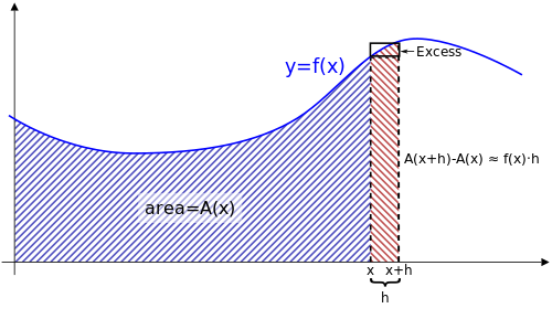
The first fundamental theorem may be interpreted as follows. Given a continuous function ${\displaystyle y=f(x)}$ whose graph is plotted as a curve, one defines a corresponding "area function" ${\displaystyle x\mapsto A(x)}$ such that A(x) is the area beneath the curve between 0 and x. The area A(x) may not be easily computable, but it is assumed to be well defined.

The area under the curve between x and x + h could be computed by finding the area between 0 and x + h, then subtracting the area between 0 and x. In other words, the area of this "strip" would be A(x + h) − A(x).

There is another way to estimate the area of this same strip. As shown in the accompanying figure, h is multiplied by f(x) to find the area of a rectangle that is approximately the same size as this strip. So:

In fact, this estimate becomes a perfect equality if we add the red "Excess" area in the diagram. So:

Rearranging terms:

As h approaches 0 in the limit, the last fraction must go to zero.^[6] To see this, note that the excess region is inside the tiny black-bordered rectangle, giving an upper bound for the excess area:

${\displaystyle |{\text{Excess}}|\leq h\,(f(x{+}h_{1})-f(x{+}h_{2})),}$

where ${\displaystyle x+h_{1}}$ and ${\displaystyle x+h_{2}}$ are points where f reaches its maximum and its minimum, respectively, in the interval [x, x + h].

Thus:

By the continuity of f, the right-hand expression tends to zero as h does. Therefore, the left-hand side also tends to zero, and:

That is, the derivative of the area function A(x) exists and is equal to the original function f(x), so the area function is an antiderivative of the original function.

Thus, the derivative of the integral of a function (the area) is the original function, so that derivative and integral are inverse operations which reverse each other. This is the essence of the Fundamental Theorem.

Physical intuition

Intuitively, the fundamental theorem states that integration and differentiation are essentially inverse operations which reverse each other.

The second fundamental theorem says that the sum of infinitesimal changes in a quantity over time (the integral of the derivative of the quantity) adds up to the net change in the quantity. To visualize this, imagine traveling in a car and wanting to know the distance traveled (the net change in position along the highway). You can see the velocity on the speedometer but cannot look out to see your location. Each second, you can find how far the car has traveled using distance = speed × time, multiplying the current speed (in kilometers or miles per hour) by the time interval (1 second = ${\displaystyle {\tfrac {1}{3600}}}$ hour). Summing up all these small steps, you can calculate the total distance traveled, without ever looking outside the car:

As ${\displaystyle \Delta t}$ becomes infinitesimally small, the summing up corresponds to integration. Thus, the integral of the velocity function (the derivative of position) computes how far the car has traveled (the net change in position).

The first fundamental theorem says that any quantity is the rate of change (the derivative) of the integral of the quantity from a fixed time up to a variable time. Continuing the above example, if you imagine a velocity function, you can integrate it from the starting time up to any given time to obtain a distance function whose derivative is the given velocity. (To obtain the highway-marker position, you need to add your starting position to this integral.)

Formal statements

There are two parts to the theorem. The first part deals with the derivative of an antiderivative, while the second part deals with the relationship between antiderivatives and definite integrals.

First part

This part is sometimes referred to as the first fundamental theorem of calculus.^[7]

Let f be a continuous real-valued function defined on a closed interval [a, b]. Let F be the function defined, for all x in [a, b], by

Then F is uniformly continuous on [a, b] and differentiable on the open interval (a, b), and

for all x in (a, b) so F is an antiderivative of f.

Corollary

The fundamental theorem is often employed to compute the definite integral of a function ${\displaystyle f}$ for which an antiderivative ${\displaystyle F}$ is known. Specifically, if ${\displaystyle f}$ is a real-valued continuous function on ${\displaystyle [a,b]}$ and ${\displaystyle F}$ is an antiderivative of ${\displaystyle f}$ in ${\displaystyle [a,b]}$, then

The corollary assumes continuity on the whole interval. This result is strengthened slightly in the following part of the theorem.

Second part

This part is sometimes referred to as the second fundamental theorem of calculus^[8] or the Newton–Leibniz theorem.

Let ${\displaystyle f}$ be a real-valued function on a closed interval ${\displaystyle [a,b]}$ and ${\displaystyle F}$ a continuous function on ${\displaystyle [a,b]}$ which is an antiderivative of ${\displaystyle f}$ in ${\displaystyle (a,b)}$:

If ${\displaystyle f}$ is Riemann integrable on ${\displaystyle [a,b]}$ then

The second part is somewhat stronger than the corollary because it does not assume that ${\displaystyle f}$ is continuous.

When an antiderivative ${\displaystyle F}$ of ${\displaystyle f}$ exists, then there are infinitely many antiderivatives for ${\displaystyle f}$, obtained by adding an arbitrary constant to ${\displaystyle F}$. Also, by the first part of the theorem, antiderivatives of ${\displaystyle f}$ always exist when ${\displaystyle f}$ is continuous.

Proof of the first part

For a given function f, define the function F(x) as

For any two numbers x₁ and x₁ + Δx in [a, b], we have

the latter equality resulting from the basic properties of integrals and the additivity of areas.

According to the mean value theorem for integration, there exists a real number ${\displaystyle c\in [x_{1},x_{1}+\Delta x]}$ such that

It follows that

and thus that

Taking the limit as ${\displaystyle \Delta x\to 0,}$ and keeping in mind that ${\displaystyle c\in [x_{1},x_{1}+\Delta x],}$ one gets

that is, according to the definition of the derivative, the continuity of f, and the squeeze theorem.^[9]

Proof of the corollary

Suppose F is an antiderivative of f, with f continuous on [a, b]. Let

By the first part of the theorem, we know G is also an antiderivative of f. Since F′ − G′ = 0 the mean value theorem implies that F − G is a constant function, that is, there is a number c such that G(x) = F(x) + c for all x in [a, b]. Letting x = a, we have

which means c = −F(a). In other words, G(x) = F(x) − F(a), and so

Proof of the second part

This is a limit proof by Riemann sums.

To begin, we recall the mean value theorem. Stated briefly, if F is continuous on the closed interval [a, b] and differentiable on the open interval (a, b), then there exists some c in (a, b) such that

Let f be (Riemann) integrable on the interval [a, b], and let f admit an antiderivative F on (a, b) such that F is continuous on [a, b]. Begin with the quantity F(b) − F(a). Let there be numbers x₀, ..., x_n such that

It follows that

Now, we add each F(x_i) along with its additive inverse, so that the resulting quantity is equal:

The above quantity can be written as the following sum:

$${\displaystyle F(b)-F(a)=\sum _{i=1}^{n}[F(x_{i})-F(x_{i-1})].}$$

(1')

The function F is differentiable on the interval (a, b) and continuous on the closed interval [a, b]; therefore, it is also differentiable on each interval (x_i−1, x_i) and continuous on each interval [x_i−1, x_i]. According to the mean value theorem (above), for each i there exists a ${\displaystyle c_{i}}$ in (x_i−1, x_i) such that

Substituting the above into (1'), we get

The assumption implies ${\displaystyle F'(c_{i})=f(c_{i}).}$ Also, ${\displaystyle x_{i}-x_{i-1}}$ can be expressed as ${\displaystyle \Delta x}$ of partition ${\displaystyle i}$.

$${\displaystyle F(b)-F(a)=\sum _{i=1}^{n}[f(c_{i})(\Delta x_{i})].}$$

(2')

We are describing the area of a rectangle, with the width times the height, and we are adding the areas together. Each rectangle, by virtue of the mean value theorem, describes an approximation of the curve section it is drawn over. Also ${\displaystyle \Delta x_{i}}$ need not be the same for all values of i, or in other words that the width of the rectangles can differ. What we have to do is approximate the curve with n rectangles. Now, as the size of the partitions get smaller and n increases, resulting in more partitions to cover the space, we get closer and closer to the actual area of the curve.

By taking the limit of the expression as the norm of the partitions approaches zero, we arrive at the Riemann integral. We know that this limit exists because f was assumed to be integrable. That is, we take the limit as the largest of the partitions approaches zero in size, so that all other partitions are smaller and the number of partitions approaches infinity.

So, we take the limit on both sides of (2'). This gives us

Neither F(b) nor F(a) is dependent on ${\displaystyle \|\Delta x_{i}\|}$, so the limit on the left side remains F(b) − F(a).

The expression on the right side of the equation defines the integral over f from a to b. Therefore, we obtain

which completes the proof.

Relationship between the parts

As discussed above, a slightly weaker version of the second part follows from the first part.

Similarly, it almost looks like the first part of the theorem follows directly from the second. That is, suppose G is an antiderivative of f. Then by the second theorem, ${\textstyle G(x)-G(a)=\int _{a}^{x}f(t)\,dt}$. Now, suppose ${\textstyle F(x)=\int _{a}^{x}f(t)\,dt=G(x)-G(a)}$. Then F has the same derivative as G, and therefore F′ = f. This argument only works, however, if we already know that f has an antiderivative, and the only way we know that all continuous functions have antiderivatives is by the first part of the Fundamental Theorem.^[10] For example, if f(x) = e^−x2, then f has an antiderivative, namely

and there is no simpler expression for this function. It is therefore important not to interpret the second part of the theorem as the definition of the integral. Indeed, there are many functions that are integrable but lack elementary antiderivatives, and discontinuous functions can be integrable but lack any antiderivatives at all. Conversely, many functions that have antiderivatives are not Riemann integrable (see Volterra's function).

Examples

Computing a particular integral

Suppose the following is to be calculated:

Here, ${\displaystyle f(x)=x^{2}}$ and we can use ${\textstyle F(x)={\frac {1}{3}}x^{3}}$ as the antiderivative. Therefore:

Using the first part

Suppose

is to be calculated. Using the first part of the theorem with ${\displaystyle f(t)=t^{3}}$ gives

This can also be checked using the second part of the theorem. Specifically, ${\textstyle F(t)={\frac {1}{4}}t^{4}}$ is an antiderivative of ${\displaystyle f(t)}$, so

An integral where the corollary is insufficient

Suppose

Then ${\displaystyle f(x)}$ is not continuous at zero. Moreover, this is not just a matter of how ${\displaystyle f}$ is defined at zero, since the limit as ${\displaystyle x\to 0}$ of ${\displaystyle f(x)}$ does not exist. Therefore, the corollary cannot be used to compute But consider the function Notice that ${\displaystyle F(x)}$ is continuous on ${\displaystyle [0,1]}$ (including at zero by the squeeze theorem), and ${\displaystyle F(x)}$ is differentiable on ${\displaystyle (0,1)}$ with ${\displaystyle F'(x)=f(x).}$ Therefore, part two of the theorem applies, and

Theoretical example

The theorem can be used to prove that

Since,

the result follows from,

Generalizations

The function f does not have to be continuous over the whole interval. Part I of the theorem then says: if f is any Lebesgue integrable function on [a, b] and x₀ is a number in [a, b] such that f is continuous at x₀, then

is differentiable for x = x₀ with F′(x₀) = f(x₀). We can relax the conditions on f still further and suppose that it is merely locally integrable. In that case, we can conclude that the function F is differentiable almost everywhere and F′(x) = f(x) almost everywhere. On the real line this statement is equivalent to Lebesgue's differentiation theorem. These results remain true for the Henstock–Kurzweil integral, which allows a larger class of integrable functions.^[11]

In higher dimensions Lebesgue's differentiation theorem generalizes the Fundamental theorem of calculus by stating that for almost every x, the average value of a function f over a ball of radius r centered at x tends to f(x) as r tends to 0.

Part II of the theorem is true for any Lebesgue integrable function f, which has an antiderivative F (not all integrable functions do, though). In other words, if a real function F on [a, b] admits a derivative f(x) at every point x of [a, b] and if this derivative f is Lebesgue integrable on [a, b], then^[12]

This result may fail for continuous functions F that admit a derivative f(x) at almost every point x, as the example of the Cantor function shows. However, if F is absolutely continuous, it admits a derivative F′(x) at almost every point x, and moreover F′ is integrable, with F(b) − F(a) equal to the integral of F′ on [a, b]. Conversely, if f is any integrable function, then F as given in the first formula will be absolutely continuous with F′ = f almost everywhere.

The conditions of this theorem may again be relaxed by considering the integrals involved as Henstock–Kurzweil integrals. Specifically, if a continuous function F(x) admits a derivative f(x) at all but countably many points, then f(x) is Henstock–Kurzweil integrable and F(b) − F(a) is equal to the integral of f on [a, b]. The difference here is that the integrability of f does not need to be assumed.^[13]

The version of Taylor's theorem, which expresses the error term as an integral, can be seen as a generalization of the fundamental theorem.

There is a version of the theorem for complex functions: suppose U is an open set in C and f : U → C is a function that has a holomorphic antiderivative F on U. Then for every curve γ : [a, b] → U, the curve integral can be computed as

The fundamental theorem can be generalized to curve and surface integrals in higher dimensions and on manifolds. One such generalization offered by the calculus of moving surfaces is the time evolution of integrals. The most familiar extensions of the fundamental theorem of calculus in higher dimensions are the divergence theorem and the gradient theorem.

One of the most powerful generalizations in this direction is Stokes' theorem (sometimes known as the fundamental theorem of multivariable calculus):^[14] Let M be an oriented piecewise smooth manifold of dimension n and let ${\displaystyle \omega }$ be a smooth compactly supported (n − 1)-form on M. If ∂M denotes the boundary of M given its induced orientation, then

Here d is the exterior derivative, which is defined using the manifold structure only.

The theorem is often used in situations where M is an embedded oriented submanifold of some bigger manifold (e.g. R^k) on which the form ${\displaystyle \omega }$ is defined.

The fundamental theorem of calculus allows us to pose a definite integral as a first-order ordinary differential equation.

can be posed as with ${\displaystyle y(b)}$ as the value of the integral.

See also

• Differentiation under the integral sign
• Telescoping series
• Fundamental theorem of calculus for line integrals
• Notation for differentiation

Notes

References

Bibliography

Further reading

External links

• "Fundamental theorem of calculus", Encyclopedia of Mathematics, EMS Press, 2001 [1994]
• James Gregory's Euclidean Proof of the Fundamental Theorem of Calculus at Convergence
• Isaac Barrow's proof of the Fundamental Theorem of Calculus
• Fundamental Theorem of Calculus at imomath.com
• Alternative proof of the fundamental theorem of calculus
• Fundamental Theorem of Calculus MIT.
• Fundamental Theorem of Calculus Mathworld.

References

- ^ Weisstein, Eric W. "First Fundamental Theorem of Calculus". mathworld.wolfram.com. Retrieved 2024-04-15.
- ^ Malet, Antoni (1993). "James Gregorie on tangents and the "Taylor" rule for series expansions". Archive for History of Exact Sciences. 46 (2). Springer-Verlag: 97–137. doi:10.1007/BF00375656. S2CID 120101519.
Gregorie's thought, on the other hand, belongs to a conceptual framework strongly geometrical in character. (page 137)
- ^ See, e.g., Marlow Anderson, Victor J. Katz, Robin J. Wilson, Sherlock Holmes in Babylon and Other Tales of Mathematical History, Mathematical Association of America, 2004, p. 114.
- ^ Gregory, James (1668). Geometriae Pars Universalis. Museo Galileo: Patavii: typis heredum Pauli Frambotti.
- ^ Child, James Mark; Barrow, Isaac (1916). The Geometrical Lectures of Isaac Barrow. Chicago: Open Court Publishing Company.
- ^ Bers, Lipman. Calculus, pp. 180–181 (Holt, Rinehart and Winston (1976).
- ^ Apostol 1967, §5.1
- ^ Apostol 1967, §5.3
- ^ Leithold, L. (1996), The calculus of a single variable (6th ed.), New York: HarperCollins College Publishers, p. 380.
- ^ Spivak, Michael (1980), Calculus (2nd ed.), Houston, Texas: Publish or Perish Inc.
- ^ Bartle (2001), Thm. 4.11.
- ^ Rudin 1987, th. 7.21
- ^ Bartle (2001), Thm. 4.7.
- ^ Spivak, M. (1965). Calculus on Manifolds. New York: W. A. Benjamin. pp. 124–125. ISBN 978-0-8053-9021-6.
Bibliography

- Apostol, Tom M. (1967), Calculus, Vol. 1: One-Variable Calculus with an Introduction to Linear Algebra (2nd ed.), New York: John Wiley & Sons, ISBN 978-0-471-00005-1.
- Bartle, Robert (2001), A Modern Theory of Integration, AMS, ISBN 0-8218-0845-1.
- Leithold, L. (1996), The calculus of a single variable (6th ed.), New York: HarperCollins College Publishers.
- Rudin, Walter (1987), Real and Complex Analysis (third ed.), New York: McGraw-Hill Book Co., ISBN 0-07-054234-1