Negative hypergeometric| Probability mass function 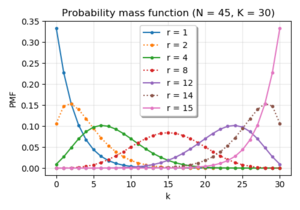 |
| Cumulative distribution function  |
| Parameters |  - total number of elements - total number of elements
 - total number of 'success' elements - total number of 'success' elements
 - number of failures when experiment is stopped - number of failures when experiment is stopped |
|---|
| Support |  - number of successes when experiment is stopped. - number of successes when experiment is stopped. |
|---|
| PMF |  |
|---|
| Mean |  |
|---|
| Variance | ![{\displaystyle r{\frac {(N+1)K}{(N-K+1)(N-K+2)}}[1-{\frac {r}{N-K+1}}]}](https://wikimedia.org/api/rest_v1/media/math/render/svg/51e440acb363f2b562dbb11e50df1f9a41a68fd9) |
|---|
In probability theory and statistics, the negative hypergeometric distribution describes probabilities for when sampling from a finite population without replacement in which each sample can be classified into two mutually exclusive categories like Pass/Fail or Employed/Unemployed. As random selections are made from the population, each subsequent draw decreases the population causing the probability of success to change with each draw. Unlike the standard hypergeometric distribution, which describes the number of successes in a fixed sample size, in the negative hypergeometric distribution, samples are drawn until  failures have been found, and the distribution describes the probability of finding
  successes in such a sample. In other words, the negative hypergeometric distribution describes the likelihood of successes in a sample with exactly failures.
Definition
There are  elements, of which
  are defined as "successes" and the rest are "failures".
Elements are drawn one after the other, without replacements, until failures are encountered. Then, the drawing stops and the number of successes is counted. The negative hypergeometric distribution,  is the discrete distribution of this .
[1]
The negative hypergeometric distribution is a special case of the beta-binomial distribution[2] with parameters  and
and  both being integers (and
  ).
).
The outcome requires that we observe successes in  draws and the
  bit must be a failure. The probability of the former can be found by the direct application of the hypergeometric distribution
  and the probability of the latter is simply the number of failures remaining
  divided by the size of the remaining population
  . The probability of having exactly successes up to the
  failure (i.e. the drawing stops as soon as the sample includes the predefined number of failures) is then the product of these two probabilities:

Therefore, a random variable  follows the negative hypergeometric distribution if its probability mass function (pmf) is given by

where
- is the population size,
- is the number of success states in the population,
- is the number of failures,
- is the number of observed successes,
 is a binomial coefficient
By design the probabilities sum up to 1. However, in case we want show it explicitly we have:

where we have used that,

which can be derived using the binomial identity,

and the Chu–Vandermonde identity,

which holds for any complex-values  and
and  and any non-negative integer .
Expectation
When counting the number of successes before failures, the expected number of successes is  and can be derived as follows.
![{\displaystyle {\begin{aligned}E[X]&=\sum _{k=0}^{K}k\Pr(X=k)=\sum _{k=0}^{K}k{\frac {{{k+r-1} \choose {k}}{{N-r-k} \choose {K-k}}}{N \choose K}}={\frac {r}{N \choose K}}\left[\sum _{k=0}^{K}{\frac {(k+r)}{r}}{{k+r-1} \choose {r-1}}{{N-r-k} \choose {K-k}}\right]-r\\&={\frac {r}{N \choose K}}\left[\sum _{k=0}^{K}{{k+r} \choose {r}}{{N-r-k} \choose {K-k}}\right]-r={\frac {r}{N \choose K}}\left[\sum _{k=0}^{K}{{k+r} \choose {k}}{{N-r-k} \choose {K-k}}\right]-r\\&={\frac {r}{N \choose K}}\left[{{N+1} \choose K}\right]-r={\frac {rK}{N-K+1}},\end{aligned}}}](https://wikimedia.org/api/rest_v1/media/math/render/svg/34e659bf96fe9a5fd5828d3e0b3fe1f5c6489d00)
where we have used the relationship  , that we derived above to show that the negative hypergeometric distribution was properly normalized.
Variance
The variance can be derived by the following calculation.
![{\displaystyle {\begin{aligned}E[X^{2}]&=\sum _{k=0}^{K}k^{2}\Pr(X=k)=\left[\sum _{k=0}^{K}(k+r)(k+r+1)\Pr(X=k)\right]-(2r+1)E[X]-r^{2}-r\\&={\frac {r(r+1)}{N \choose K}}\left[\sum _{k=0}^{K}{{k+r+1} \choose {r+1}}{{N+1-(r+1)-k} \choose {K-k}}\right]-(2r+1)E[X]-r^{2}-r\\&={\frac {r(r+1)}{N \choose K}}\left[{{N+2} \choose K}\right]-(2r+1)E[X]-r^{2}-r={\frac {rK(N-r+Kr+1)}{(N-K+1)(N-K+2)}}\end{aligned}}}](https://wikimedia.org/api/rest_v1/media/math/render/svg/77aa81b3335fd171000929e5e6e74bb9c94a44b3)
Then the variance is ![{\displaystyle {\textrm {Var}}[X]=E[X^{2}]-\left(E[X]\right)^{2}={\frac {rK(N+1)(N-K-r+1)}{(N-K+1)^{2}(N-K+2)}}}](https://wikimedia.org/api/rest_v1/media/math/render/svg/ec84a94aaf05ac30602871150e31225388300cf9)
Related distributions
If the drawing stops after a constant number of draws (regardless of the number of failures), then the number of successes has the hypergeometric distribution,  . The two functions are related in the following way:[1]

Negative-hypergeometric distribution (like the hypergeometric distribution) deals with draws without replacement, so that the probability of success is different in each draw. In contrast, negative-binomial distribution (like the binomial distribution) deals with draws with replacement, so that the probability of success is the same and the trials are independent. The following table summarizes the four distributions related to drawing items:
| With replacements | No replacements |
| # of successes in constant # of draws | binomial distribution | hypergeometric distribution |
| # of successes in constant # of failures | negative binomial distribution | negative hypergeometric distribution |
Some authors[3][4] define the negative hypergeometric distribution to be the number of draws required to get the th failure. If we let  denote this number then it is clear that
  where is as defined above. Hence the PMF

If we let the number of failures  be denoted by
  means that we have

The support of is the set  . It is clear that:
![{\displaystyle E[Y]=E[X]+r={\frac {r(N+1)}{M+1}}}](https://wikimedia.org/api/rest_v1/media/math/render/svg/05ecb17d532fb5fae1a0035199a0f7d9bd302d6d)
and ![{\displaystyle {\textrm {Var}}[X]={\textrm {Var}}[Y]}](https://wikimedia.org/api/rest_v1/media/math/render/svg/b3fc52f9aa4005d8143f0d6ce4a288b41f9fc32a) .
.
References
- ^ a b Negative hypergeometric distribution in Encyclopedia of Math.
- ^ Johnson, Norman L.; Kemp, Adrienne W.; Kotz, Samuel (2005). Univariate Discrete Distributions. Wiley. ISBN 0-471-27246-9. §6.2.2 (p.253–254)
- ^ Rohatgi, Vijay K., and AK Md Ehsanes Saleh. An introduction to probability and statistics. John Wiley & Sons, 2015.
- ^ Khan, RA (1994). A note on the generating function of a negative hypergeometric distribution. Sankhya: The Indian Journal of Statistics B, 56(3), 309-313.
Probability distributions (
list)
Discrete
univariate | with finite
support | |
|---|
with infinite
support | |
|---|
|
|---|
Continuous
univariate | supported on a
bounded interval | |
|---|
supported on a
semi-infinite
interval | |
|---|
supported
on the whole
real line | |
|---|
with support
whose type varies | |
|---|
|
|---|
Mixed
univariate | |
|---|
Multivariate
(joint) | |
|---|
| Directional | |
|---|
Degenerate
and singular | |
|---|
| Families | |
|---|
 Category Category Commons Commons
|


