Atan2

In computing and mathematics, the function atan2 is the 2-argument arctangent. By definition, ${\displaystyle \theta =\operatorname {atan2} (y,x)}$ is the angle measure (in radians, with ${\displaystyle -\pi <\theta \leq \pi }$) between the positive ${\displaystyle x}$-axis and the ray from the origin to the point ${\displaystyle (x,\,y)}$ in the Cartesian plane. Equivalently, ${\displaystyle \operatorname {atan2} (y,x)}$ is the argument (also called phase or angle) of the complex number ${\displaystyle x+iy.}$

The ${\displaystyle \operatorname {atan2} }$ function first appeared in the programming language Fortran in 1961. It was originally intended to return a correct and unambiguous value for the angle θ in converting from Cartesian coordinates (x, y) to polar coordinates (r, θ). If ${\displaystyle \theta =\operatorname {atan2} (y,x)}$ and ${\textstyle r={\sqrt {x^{2}+y^{2}}}}$, then ${\displaystyle x=r\cos \theta }$ and ${\displaystyle y=r\sin \theta .}$

If x > 0, the desired angle measure is ${\textstyle \theta =\operatorname {atan2} (y,x)=\arctan \left(y/x\right).}$ However, when x < 0, the angle ${\displaystyle \arctan(y/x)}$ is diametrically opposite the desired angle, and ±π (a half turn) must be added to place the point in the correct quadrant.^[1] Using the ${\displaystyle \operatorname {atan2} }$ function does away with this correction, simplifying code and mathematical formulas.

Motivation

The ordinary single-argument arctangent function only returns angle measures in the interval ${\textstyle {\left(-{\frac {\pi }{2}},+{\frac {\pi }{2}}\right)},}$ and when invoking it to find the angle measure between the x-axis and an arbitrary vector in the Cartesian plane, there is no simple way to indicate a direction in the left half-plane (that is, a point ${\displaystyle (x,\,y)}$ with ${\displaystyle x<0}$). Diametrically opposite angle measures have the same tangent because ${\displaystyle y/x=(-y)/(-x),}$ so the tangent ${\displaystyle y/x}$ is not in itself sufficient to uniquely specify an angle.

To determine an angle measure using the arctangent function given a point or vector ${\displaystyle (x,y),}$ mathematical formulas or computer code must handle multiple cases; at least one for positive values of ${\displaystyle x}$ and one for negative values of ${\displaystyle x,}$ and sometimes additional cases when ${\displaystyle y}$ is negative or one coordinate is zero. Finding angle measures and converting Cartesian to polar coordinates are common in scientific computing, and this code is redundant and error-prone.

To remedy this, computer programming languages introduced the atan2 function, at least as early as the Fortran IV language of the 1960s.^[2] The quantity atan2(y,x) is the angle measure between the x-axis and a ray from the origin to a point (x, y) anywhere in the Cartesian plane. The signs of x and y are used to determine the quadrant of the result and select the correct branch of the multivalued function Arctan(y/x).

The atan2 function is useful in many applications involving Euclidean vectors such as finding the direction from one point to another or converting a rotation matrix to Euler angles.

The atan2 function is now included in many other programming languages, and is also commonly found in mathematical formulas throughout science and engineering.

Argument order

In 1961, Fortran introduced the atan2 function with argument order ${\displaystyle (y,x)}$ so that the argument (phase angle) of a complex number is ${\displaystyle \operatorname {arg} z=\operatorname {atan2} (\operatorname {Im} z,\operatorname {Re} z).}$ This follows the left-to-right order of a fraction written ${\displaystyle y/x,}$ so that ${\displaystyle \operatorname {atan2} (y,x)=\operatorname {atan} (y/x)}$ for positive values of ${\displaystyle x.}$ However, this is the opposite of the conventional component order for complex numbers, ${\displaystyle z=x+iy,}$ or as coordinates ${\displaystyle (\operatorname {Re} z,\operatorname {Im} z).}$ See section Definition and computation.

Some other programming languages (see § Realizations of the function in common computer languages) picked the opposite order instead. For example Microsoft Excel uses ${\displaystyle \operatorname {Atan2} (x,y),}$ OpenOffice Calc uses ${\displaystyle \operatorname {arctan2} (x,y),}$ and Mathematica uses ${\displaystyle \operatorname {ArcTan} [x,y],}$ defaulting to one-argument arctangent if called with one argument.

Definition and computation

The function atan2 computes the principal value of the argument function applied to the complex number x + i y. That is, atan2(y, x) = Pr arg(x + i y) = Arg(x + i y). The argument could be changed by an arbitrary multiple of 2π (corresponding to a complete turn around the origin) without making any difference to the angle, but to define atan2 uniquely one uses the principal value in the range ${\displaystyle (-\pi ,\pi ]}$, that is, −π < atan2(y, x) ≤ π.

In terms of the standard arctan function, whose range is (−π/2, π/2), it can be expressed as follows to define a surface that has no discontinuities except along the semi-infinite line x<0 y=0:

A compact expression with four overlapping half-planes is

The Iverson bracket notation allows for an even more compact expression:^{[note 1]}

Formula without apparent conditional construct:

The following expression derived from the tangent half-angle formula can also be used to define atan2:

This expression may be more suited for symbolic use than the definition above. However it is unsuitable for general floating-point computational use, as the effect of rounding errors in ${\textstyle {\sqrt {x^{2}+y^{2}}}}$ expand near the region x < 0, y = 0 (this may even lead to a division of y by zero).

A variant of the last formula that avoids these inflated rounding errors:

Notes:

• This produces results in the range (−π, π].^{[note 2]}
• As mentioned above, the principal value of the argument atan2(y, x) can be related to arctan(y/x) by trigonometry. The derivation goes as follows:
  If (x, y) = (r cos θ, r sin θ), then tan(θ/2) = y / (r + x). It follows that
  $${\displaystyle \operatorname {atan2} (y,x)=\theta =2\,\theta /2=2\arctan {\frac {y}{{\sqrt {x^{2}+y^{2}}}+x}}.}$$

  
  Note that √x² + y² + x ≠ 0 in the domain in question.

Derivative

As the function atan2 is a function of two variables, it has two partial derivatives. At points where these derivatives exist, atan2 is, except for a constant, equal to arctan(y/x). Hence for x > 0 or y ≠ 0,

${\displaystyle {\begin{aligned}&{\frac {\partial }{\partial x}}\operatorname {atan2} (y,\,x)={\frac {\partial }{\partial x}}\arctan \left({\frac {y}{x}}\right)=-{\frac {y}{x^{2}+y^{2}}},\\[5pt]&{\frac {\partial }{\partial y}}\operatorname {atan2} (y,\,x)={\frac {\partial }{\partial y}}\arctan \left({\frac {y}{x}}\right)={\frac {x}{x^{2}+y^{2}}}.\end{aligned}}}$

Thus the gradient of atan2 is given by

${\displaystyle \nabla {\text{atan2}}(y,x)=\left({-y \over x^{2}+y^{2}},\ {x \over x^{2}+y^{2}}\right).}$

Informally representing the function atan2 as the angle function θ(x, y) = atan2(y, x) (which is only defined up to a constant) yields the following formula for the total differential:

${\displaystyle {\begin{aligned}\mathrm {d} \theta &={\frac {\partial }{\partial x}}\operatorname {atan2} (y,\,x)\,\mathrm {d} x+{\frac {\partial }{\partial y}}\operatorname {atan2} (y,\,x)\,\mathrm {d} y\\[5pt]&=-{\frac {y}{x^{2}+y^{2}}}\,\mathrm {d} x+{\frac {x}{x^{2}+y^{2}}}\,\mathrm {d} y.\end{aligned}}}$

While the function atan2 is discontinuous along the negative x-axis, reflecting the fact that angle cannot be continuously defined, this derivative is continuously defined except at the origin, reflecting the fact that infinitesimal (and indeed local) changes in angle can be defined everywhere except the origin. Integrating this derivative along a path gives the total change in angle over the path, and integrating over a closed loop gives the winding number.

In the language of differential geometry, this derivative is a one-form, and it is closed (its derivative is zero) but not exact (it is not the derivative of a 0-form, i.e., a function), and in fact it generates the first de Rham cohomology of the punctured plane. This is the most basic example of such a form, and it is fundamental in differential geometry.

The partial derivatives of atan2 do not contain trigonometric functions, making it particularly useful in many applications (e.g. embedded systems) where trigonometric functions can be expensive to evaluate.

Illustrations

This figure shows values of atan2 along selected rays from the origin, labelled at the unit circle. The values, in radians, are shown inside the circle. The diagram uses the standard mathematical convention that angles increase counterclockwise from zero along the ray to the right. Note that the order of arguments is reversed; the function atan2(y, x) computes the angle corresponding to the point (x, y).

This figure shows the values of ${\displaystyle \arctan(\tan(\theta ))}$ along with ${\displaystyle \operatorname {atan2} (\sin(\theta ),\cos(\theta ))}$ for ${\displaystyle 0\leq \theta \leq 2\pi }$. Both functions are odd and periodic with periods ${\displaystyle \pi }$ and ${\displaystyle 2\pi }$, respectively, and thus can easily be supplemented to any region of real values of ${\displaystyle \theta }$. One can clearly see the branch cuts of the ${\displaystyle \operatorname {atan2} }$-function at ${\displaystyle \theta =\pi }$, and of the ${\displaystyle \arctan }$-function at ${\displaystyle \theta \in \{{\tfrac {\pi }{2}},\;{\tfrac {3\pi }{2}}\}}$.^[3]

The two figures below show 3D views of respectively atan2(y, x) and arctan(y/x) over a region of the plane. Note that for atan2(y, x), rays in the X/Y-plane emanating from the origin have constant values, but for arctan(y/x) lines in the X/Y-plane passing through the origin have constant values. For x > 0, the two diagrams give identical values.

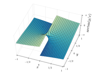Angle sum and difference identity

Sums of ${\displaystyle \operatorname {atan2} }$ may be collapsed into a single operation according to the following identity

${\displaystyle \operatorname {atan2} (y_{1},x_{1})\pm \operatorname {atan2} (y_{2},x_{2})=\operatorname {atan2} (y_{1}x_{2}\pm y_{2}x_{1},x_{1}x_{2}\mp y_{1}y_{2})}$

...provided that ${\displaystyle \operatorname {atan2} (y_{1},x_{1})\pm \operatorname {atan2} (y_{2},x_{2})\in (-\pi ,\pi ]}$.

The proof involves considering two cases, one where ${\displaystyle y_{2}\neq 0}$ or ${\displaystyle x_{2}>0}$ and one where ${\displaystyle y_{2}=0}$ and ${\displaystyle x_{2}<0}$.

We only consider the case where ${\displaystyle y_{2}\neq 0}$ or ${\displaystyle x_{2}>0}$. To start, we make the following observations:

1. ${\displaystyle -\operatorname {atan2} (y,x)=\operatorname {atan2} (-y,x)}$ provided that ${\displaystyle y\neq 0}$ or ${\displaystyle x>0}$.
2. ${\displaystyle \operatorname {Arg} (x+iy)=\operatorname {atan2} (y,x)}$, where ${\displaystyle \operatorname {Arg} }$ is the complex argument function.
3. ${\displaystyle \theta =\operatorname {Arg} e^{i\theta }}$ whenever ${\displaystyle \theta \in (-\pi ,\pi ]}$, a consequence of Euler's formula.
4. ${\displaystyle \operatorname {Arg} (e^{i\operatorname {Arg} \zeta _{1}}e^{i\operatorname {Arg} \zeta _{2}})=\operatorname {Arg} (\zeta _{1}\zeta _{2})}$.

To see (4), we have the identity ${\displaystyle e^{i\operatorname {Arg} \zeta }={\bar {\zeta }}}$ where ${\displaystyle {\bar {\zeta }}=\zeta /\left|\zeta \right|}$, hence ${\displaystyle \operatorname {Arg} (e^{i\operatorname {Arg} \zeta _{1}}e^{i\operatorname {Arg} \zeta _{2}})=\operatorname {Arg} ({\bar {\zeta _{1}}}{\bar {\zeta _{2}}})}$. Furthermore, since ${\displaystyle \operatorname {Arg} \zeta =\operatorname {Arg} a\zeta }$ for any positive real value ${\displaystyle a}$, then if we let ${\displaystyle \zeta =\zeta _{1}\zeta _{2}}$ and ${\displaystyle a={\frac {1}{\left|\zeta _{1}\right|\left|\zeta _{2}\right|}}}$ then we have ${\displaystyle \operatorname {Arg} ({\bar {\zeta _{1}}}{\bar {\zeta _{2}}})=\operatorname {Arg} (\zeta _{1}\zeta _{2})}$.

From these observations have following equivalences:

${\displaystyle {\begin{aligned}\operatorname {atan2} (y_{1},x_{1})\pm \operatorname {atan2} (y_{2},x_{2})&{}=\operatorname {atan2} (y_{1},x_{1})+\operatorname {atan2} (\pm y_{2},x_{2})&{\text{by (1)}}\\&{}=\operatorname {Arg} (x_{1}+iy_{1})+\operatorname {Arg} (x_{2}\pm iy_{2})&{\text{by (2)}}\\&{}=\operatorname {Arg} e^{i(\operatorname {Arg} (x_{1}+iy_{1})+\operatorname {Arg} (x_{2}\pm iy_{2}))}&{\text{by (3)}}\\&{}=\operatorname {Arg} (e^{i\operatorname {Arg} (x_{1}+iy_{1})}e^{i\operatorname {Arg} (x_{2}\pm iy_{2})})\\&{}=\operatorname {Arg} ((x_{1}+iy_{1})(x_{2}\pm iy_{2}))&{\text{by (4)}}\\&{}=\operatorname {Arg} (x_{1}x_{2}\mp y_{1}y_{2}+i(y_{1}x_{2}\pm y_{2}x_{1}))\\&{}=\operatorname {atan2} (y_{1}x_{2}\pm y_{2}x_{1},x_{1}x_{2}\mp y_{1}y_{2})&{\text{by (2)}}\end{aligned}}}$

Corollary: if ${\displaystyle (y_{1},x_{1})}$ and ${\displaystyle (y_{2},x_{2})}$ are 2-dimensional vectors, the difference formula is frequently used in practice to compute the angle between those vectors with the help of ${\displaystyle \operatorname {atan2} }$, since the resulting computation behaves benign in the range ${\displaystyle (-\pi ,\pi ]}$ and can thus be used without range checks in many practical situations.

East-counterclockwise, north-clockwise and south-clockwise conventions, etc.

The ${\displaystyle \mathrm {atan2} }$ function was originally designed for the convention in pure mathematics that can be termed east-counterclockwise. In practical applications, however, the north-clockwise and south-clockwise conventions are often the norm. In atmospheric sciences, for instance, the wind direction can be calculated using the ${\displaystyle \mathrm {atan2} }$ function with the east- and north-components of the wind vector as its arguments;^[4] the solar azimuth angle can be calculated similarly with the east- and north-components of the solar vector as its arguments. The wind direction is normally defined in the north-clockwise sense, and the solar azimuth angle uses both the north-clockwise and south-clockwise conventions widely.^[5] These different conventions can be realized by swapping the positions and changing the signs of the x- and y-arguments as follows:

• ${\displaystyle \mathrm {atan2} (y,x),\;\;\;\;\;}$ (East-Counterclockwise Convention)
• ${\displaystyle \mathrm {atan2} (x,y),\;\;\;\;\;}$ (North-Clockwise Convention)
• ${\displaystyle \mathrm {atan2} (-x,-y)}$. (South-Clockwise Convention)

As an example, let ${\displaystyle x_{0}={\frac {\sqrt {3}}{2}}}$ and ${\displaystyle y_{0}={\frac {1}{2}}}$, then the east-counterclockwise format gives ${\displaystyle \mathrm {atan2} (y_{0},x_{0})\cdot {\frac {180}{\pi }}=30^{\circ }}$, the north-clockwise format gives ${\displaystyle \mathrm {atan2} (x_{0},y_{0})\cdot {\frac {180}{\pi }}=60^{\circ }}$, and the south-clockwise format gives ${\displaystyle \mathrm {atan2} (-x_{0},-y_{0})\cdot {\frac {180}{\pi }}=-120^{\circ }}$.

Changing the sign of the x- and/or y-arguments and/or swapping their positions can create 8 possible variations of the ${\displaystyle \mathrm {atan2} }$ function and they, interestingly, correspond to 8 possible definitions of the angle, namely, clockwise or counterclockwise starting from each of the 4 cardinal directions, north, east, south and west.

Realizations of the function in common computer languages

The realization of the function differs from one computer language to another:

• In Microsoft Excel,^[6] OpenOffice.org Calc, LibreOffice Calc,^[7] Google Spreadsheets,^[8] iWork Numbers,^[9] and ANSI SQL:2008 standard,^[10] the 2-argument arctangent function has the two arguments in the standard sequence ${\displaystyle (\operatorname {Re} ,\operatorname {Im} )}$ (reversed relative to the convention used in the discussion above).
• In Mathematica, the form ArcTan[x, y] is used where the one parameter form supplies the normal arctangent. Mathematica classifies ArcTan[0, 0] as an indeterminate expression.
• On most TI graphing calculators (excluding the TI-85 and TI-86), the equivalent function is called R►Pθ and has the arguments ${\displaystyle (\operatorname {Re} ,\operatorname {Im} )}$.
• On TI-85 the arg function is called angle(x,y) and although it appears to take two arguments, it really only has one complex argument which is denoted by a pair of numbers: x + i y = (x, y).

The ${\displaystyle (\operatorname {Im} ,\operatorname {Re} )}$ convention is used by:

• The C function atan2, and most other computer implementations, are designed to reduce the effort of transforming cartesian to polar coordinates and so always define atan2(0, 0). On implementations without signed zero, or when given positive zero arguments, it is normally defined as 0. It will always return a value in the range [−π, π] rather than raising an error or returning a NaN (Not a Number).
• In Common Lisp, where optional arguments exist, the atan function allows one to optionally supply the x coordinate: (atan y x).^[11]
• In Julia, the situation is similar to Common Lisp: instead of atan2, the language has a one-parameter and a two-parameter form for atan.^[12] However, it has many more than two methods, to allow for aggressive optimisation at compile time (see the section "Why don't you compile Matlab/Python/R/… code to Julia?" ^[13]).
• For systems implementing signed zero, infinities, or Not a Number (for example, IEEE floating point), it is common to implement reasonable extensions which may extend the range of values produced to include −π and −0 when y = −0. These also may return NaN or raise an exception when given a NaN argument.
• In the Intel x86 Architecture assembler code, atan2 is known as the FPATAN (floating-point partial arctangent) instruction.^[14] It can deal with infinities and results lie in the closed interval [−π, π], e.g. atan2(∞, x) = +π/2 for finite x. Particularly, FPATAN is defined when both arguments are zero:

  atan2(+0, +0) = +0;

  atan2(+0, −0) = +π;

  atan2(−0, +0) = −0;

  atan2(−0, −0) = −π.

This definition is related to the concept of signed zero.

• In mathematical writings other than source code, such as in books and articles, the notations Arctan^[15] and Tan^−1[16] have been utilized; these are capitalized variants of the regular arctan and tan⁻¹. This usage is consistent with the complex argument notation, such that Atan(y, x) = Arg(x + i y).
• On HP calculators, treat the coordinates as a complex number and then take the ARG. Or << C->R ARG >> 'ATAN2' STO.
• On scientific calculators the function can often be calculated as the angle given when (x, y) is converted from rectangular coordinates to polar coordinates.
• Systems supporting symbolic mathematics normally return an undefined value for atan2(0, 0) or otherwise signal that an abnormal condition has arisen.
• The free math library FDLIBM (Freely Distributable LIBM) available from netlib has source code showing how it implements atan2 including handling the various IEEE exceptional values.
• For systems without a hardware multiplier the function atan2 can be implemented in a numerically reliable manner by the CORDIC method. Thus implementations of atan(y) will probably choose to compute atan2(y, 1).

See also

• hypot

References

External links

• ATAN2 Online calculator
• Java 1.6 SE JavaDoc
• atan2 at Everything2
• PicBasic Pro solution atan2 for a PIC18F

Other implementations/code for atan2

• "Bearing Between Two Points". Archived from the original on 18 November 2020. Retrieved 21 February 2022.

• "Arctan and Polar Coordinates". Archived from the original on 18 October 2018. Retrieved 21 February 2022.

• "What's 'Arccos'?". Archived from the original on 6 September 2017. Retrieved 21 February 2022.

Notes

References

- ^ "The argument of a complex number" (PDF). Santa Cruz Institute for Particle Physics. Winter 2011.
- ^ Organick, Elliott I. (1966). A FORTRAN IV Primer. Addison-Wesley. p. 42.
Some processors also offer the library function called ATAN2, a function of two arguments (opposite and adjacent).
- ^ "Wolf Jung: Mandel, software for complex dynamics". www.mndynamics.com. Retrieved 20 April 2018.
- ^ "Wind Direction Quick Reference". NCAR UCAR Earth Observing Laboratory.
- ^ Zhang, Taiping; Stackhouse, Paul W.; MacPherson, Bradley; Mikovitz, J. Colleen (2021). "A solar azimuth formula that renders circumstantial treatment unnecessary without compromising mathematical rigor: Mathematical setup, application and extension of a formula based on the subsolar point and atan2 function". Renewable Energy. 172: 1333–1340. doi:10.1016/j.renene.2021.03.047. S2CID 233631040.
- ^ "Microsoft Excel Atan2 Method". Microsoft.
- ^ "LibreOffice Calc ATAN2". Libreoffice.org.
- ^ "Functions and formulas – Docs Editors Help". support.google.com.
- ^ "Numbers' Trigonometric Function List". Apple.
- ^ "ANSI SQL:2008 standard". Teradata. Archived from the original on 2015-08-20.
- ^ "CLHS: Function ASIN, ACOS, ATAN". LispWorks.
- ^ "Mathematics · The Julia Language". docs.julialang.org.
- ^ "Frequently Asked Questions · The Julia Language". docs.julialang.org.
- ^ IA-32 Intel Architecture Software Developer’s Manual. Volume 2A: Instruction Set Reference, A-M, 2004.
- ^ Burger, Wilhelm; Burge, Mark J. (7 July 2010). Principles of Digital Image Processing: Fundamental Techniques. Springer Science & Business Media. ISBN 978-1-84800-191-6. Retrieved 20 April 2018 – via Google Books.
- ^ Glisson, Tildon H. (18 February 2011). Introduction to Circuit Analysis and Design. Springer Science & Business Media. ISBN 9789048194438. Retrieved 20 April 2018 – via Google Books.